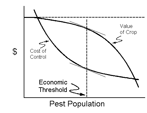


EIL = C/(VIDK)
where:
EIL = economic injury level
C = cost of insect control
V = value of a unit of the crop
I = injury units per insect
D = damage (proportion of yield lost) per injury unit
K = proportionate reduction in injury
This equation expands the simple proportion of yield lost per insect into a term for "Injury", which represents the physiological effects of insect feeding, "damage", which is a measurable loss in yield or quality per unit of injury, and a dimensionless constant, K, which represents the proportionate reduction in injury as the result of the insect control.
- Real management situations are rarely
that simple
- We usually have to consider several
management variables, all of which
simultaneously affect crop yield
- And/or we might have to make these decisions at several times throughout the season
- To maximize something or to minimize
something
- e.g., to maximize yields, maximize
profits, minimize effort, or minimize
costs
- It is possible to optimize only one
objective at a time
- The solution(s) is/are the combination of decision variables that optimizes the objective

- Unfortunately in this example the more
resistant varieties have either a lower
quality or lower yield than the most
susceptible one
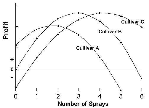
- Execute the simulation with a range of
fungicide levels (number of sprays per
season) for each of the cultivars
- Using the marginal analysis procedure,
determine the profit for each set of
input values
- In this example Cultivar C is the most
susceptible, and Cultivar A the least
susceptible
- In the absence of fungicides Cultivar
A would yield maximum profit
- There are two optimum solutions, 3 sprays on Cultivar B and 4 sprays on Cultivar C
- In this example Cultivar C is the most
susceptible, and Cultivar A the least
susceptible
- In this example 20 runs were required -- not unreasonable
- Suppose we had 5 cultivars, 4 different
fungicides, 3 spray schedules, 7 levels
of fungicide and wanted to look at the
mean and variance of the profit using
the past 10 seasons of weather data
- 5 x 4 x 3 x 7 x 10 = 4200 runs
- If each run cost $.50 on the supercomputer, the cost would be $2100
- If each run took 1 min on a microcomputer, it would take about 3 days of continuous computing
- 5 x 4 x 3 x 7 x 10 = 4200 runs

- Define the objective function
- Allocate weed control costs between
herbicide application and hand weeding
to maximize profit
- In this example (for simplicity) we
will make the yield and price constant
and set the total revenue at $250/acre
- Therefore, maximizing profit in this example means minimizing cost
- Allocate weed control costs between
herbicide application and hand weeding
to maximize profit
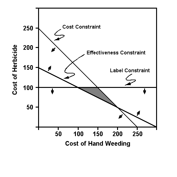
- Identify the constraints
- Cost constraint: if x is the cost of
hand weeding and y is the cost of
herbicide application, then

- Weed control effectiveness constraint:
- To achieve the yield that gives us
the above total revenue ($250), we
must invest at least $300/acre in
hand weeding
- The amount of hand weeding required
can be reduced by $2 for every $1
spent on the herbicide
- Therefore, the constraint is given by

- To achieve the yield that gives us
the above total revenue ($250), we
must invest at least $300/acre in
hand weeding
- Herbicide label constraint:
- The amount of herbicide is limited
because of possible phytotoxicity;
the cost of the maximum allowable
rate is $100/acre
- Label constraint:

- The amount of herbicide is limited
because of possible phytotoxicity;
the cost of the maximum allowable
rate is $100/acre
- Cost constraint: if x is the cost of
hand weeding and y is the cost of
herbicide application, then
- The optimum region of feasible solution
occurs where the constraint regions
overlap
- The optimum solution (if the objective is to minimize cost) occurs where a line parallel to the cost constraint line (equal costs) is as far away from the cost constraint line as possible while remaining within the optimum region
- Can handle a large number of allocation
variables (not limited to 2 dimensions
as we are on a 2-dimensional graph)
- Can handle huge numbers of constraint
functions
- The models must be linear, or at least
must be able to be approximated by
linear functions
- These models are not dynamic (allocation
through time), but they can approximate
a dynamic solution by repeating the
analysis at intervals through time
- Linear programming cannot handle stochastic models, but probability distributions can be created by repeating the analysis with different constraints that vary according to known probability distributions
- The optimum sequence of decisions is not
simply a matter of making the optimum
decision at every decision point
- The optimum sequence is often counter-intuitive

- Suppose at each decision period we have
3 possible alternatives:
- Do nothing; no cost; no insect
mortality
- Low dose of insecticide; costs
$20/acre; kills 1/3 of insects
- High dose of insecticide; costs $100/acre; kills 3/4 of insects
- Do nothing; no cost; no insect
mortality
- Further suppose that the total revenue
accumulated during a time period is
equal to $200 minus $1 times the pest population
at the beginning of the time period.
(Each insect does $1 worth of damage.)
- Suppose that the insect populations
increase 3-fold during each time period
- If we start with a pest population of
72, the accumulated profits during the
first period are as follows:
- No insecticide: $200 - 72 - 0 = $128
- Low dose: $200 - (2/3)72 - 20 = $132
- High dose: $200 - (1/4)72 - 100 = $82
- No insecticide: $200 - 72 - 0 = $128
- The pest populations at the beginning of
time period 2 are:
- No insecticide: 72 x 3 = 216
- Low dose: (2/3)72 x 3 = 144
- High dose: (1/4)72 x 3 = 54
- No insecticide: 72 x 3 = 216
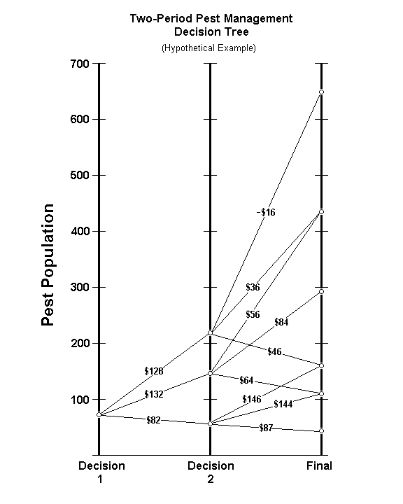
- The profits accumulated during time
period 2 and the final insect
populations are shown in the accompanying
figure
- Making the optimum decision at each
decision point would dictate using the
low dose of insecticide at each decision
point for a total profit of $132 + 84 =
$216
- However, the optimum sequence would be
to use the high dose for the first spray
and nothing for the second: $82 + 146 =
$228
- This example simply illustrates the need for a systematic optimization procedure
- For our trivial example, N = 32 = 9
- If we had 5 control alternatives and 7
decision points,
N = 57 = 78125
- The dynamic programming algorithm does not analyze all possible combinations but selects possible sets of decisions according to certain rules